Antarctic Ice Sheet — Ocean Temperature 200–500 m (Atlantic Water)

This notebook visualises the depth-averaged ocean temperature between 200 and 500 m (glc1Exp_So_t_depth4 to glc1Exp_So_t_depth8, corresponding to −210 m to −450 m) passed from the ocean model to the Antarctic Ice Sheet via the CESM coupler (cpl.hx.exp2glc files), and compares it against the EN4 observational climatology.
creation: 2026-05
contact: heig@norceresearch.no

# Import packages
import os

import numpy as np
import matplotlib.pyplot as plt
import xarray as xr

from cupid_utils.glc import utils

%matplotlib inline

Parameter configuration

Some parameters are set in CUPiD’s config.yml file, others are derived from these parameters.

# Parameter Defaults

CESM_output_dir = ""
case_name = ""  # case name
climo_nyears = 0  # number of years to load for time series
end_date = ""

base_case_output_dir = None
base_case_name = None
base_end_date = None
base_climo_nyears = 0  # number of years to load for base case time series

# Observational dataset (Atlantic Water 200-500 m)
obs_data_dir = ""  # path to Ocean_data/ais/
obs_dataset = "en4"  # only EN4 and IAP available for AIS

# Depth levels for 200-500 m AW averaging
# depth4 = -210 m, depth5 = -270 m, ..., depth8 = -450 m
aw_depth_min = 4
aw_depth_max = 8

# Climatology period for spatial map
map_climo_nyears = 30  # last N years used for climatology map and bias

# Parameters
case_name = "n1850Gaxg.n30b23LM.498.20260815"
base_case_name = ""
CESM_output_dir = "/datalake/NS9560K/noresm3/cases"
start_date = "1407-01-01"
end_date = "1456-01-01"
base_start_date = "0000-01-01"
base_end_date = "0000-01-01"
lc_kwargs = {"threads_per_worker": 1}
serial = False
obs_data_dir = "/nird/datapeak/NS9560K/users/heig/CUPiD_testdata/diagnostic_framework/Ocean_data/ais"
obs_dataset = "en4"
climo_nyears = 50
base_climo_nyears = 0
aw_depth_min = 4
aw_depth_max = 8
subset_kwargs = {}
product = "/nird/datapeak/NS9560K/users/heig/CUPiD_Apr/examples/glc_metrics/computed_notebooks//glc/Antarctica_ocean_temp_200-500m.ipynb"

# Want some base case parameter defaults to equal control case values
if base_case_name is not None:
    if base_case_output_dir is None:
        base_case_output_dir = CESM_output_dir

    if base_end_date is None:
        base_end_date = end_date

    if base_climo_nyears == 0:
        base_climo_nyears = climo_nyears

last_year = int(end_date.split("-")[0])

case_path = os.path.join(
    CESM_output_dir, case_name, "cpl", "hist"
)  # path to cpl output

if base_case_name is not None:
    base_last_year = int(base_end_date.split("-")[0])
    base_case_path = os.path.join(
        base_case_output_dir, base_case_name, "cpl", "hist"
    )  # path to cpl output

Make datasets

Read CESM ocean temperature averaged over 200–500 m and load observations.

# Load all available years for time series; climatology uses last map_climo_nyears years
ocean_temp_case = utils.read_cesm_ocean_temp_avg(
    case_path, case_name, last_year, climo_nyears,
    depth_min=aw_depth_min, depth_max=aw_depth_max, isx="AIS"
)
if ocean_temp_case is None:
    raise RuntimeError(f"AIS not present in {case_name!r} output — skipping notebook.")
ocean_temp_case_climo = ocean_temp_case.isel(time=slice(-map_climo_nyears, None)).mean("time")

if base_case_name:
    ocean_temp_base = utils.read_cesm_ocean_temp_avg(
        base_case_path, base_case_name, base_last_year, base_climo_nyears,
        depth_min=aw_depth_min, depth_max=aw_depth_max, isx="AIS"
    )
    ocean_temp_base_climo = ocean_temp_base.isel(time=slice(-map_climo_nyears, None)).mean("time")

number of years used in climatology =  50

# Spatially averaged time series (domain mean in °C)
first_year = last_year - len(ocean_temp_case["time"]) + 1
climo_first_year = last_year - map_climo_nyears + 1
avg_temp_case = ocean_temp_case.mean(["glc1Exp_ny", "glc1Exp_nx"])
avg_temp_case_climo = float(np.nanmean(ocean_temp_case_climo.data))

if base_case_name:
    base_first_year = base_last_year - len(ocean_temp_base["time"]) + 1
    base_climo_first_year = base_last_year - map_climo_nyears + 1
    avg_temp_base = ocean_temp_base.mean(["glc1Exp_ny", "glc1Exp_nx"])
    avg_temp_base_climo = float(np.nanmean(ocean_temp_base_climo.data))

# Load observational AW 200-500 m climatology (already on CISM AIS grid)
obs_file = os.path.join(obs_data_dir, "aw_200_500m", f"{obs_dataset}_aw_cism.nc")
obs_aw = utils.read_obs_ocean_temp(obs_file, "aw_temp")
obs_mean = float(np.nanmean(obs_aw.data))

Generate plots

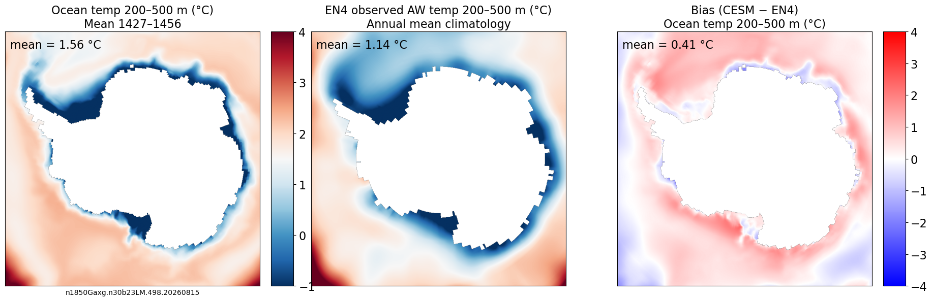
Spatial maps: CESM climatology | Observations | Bias (CESM − obs).
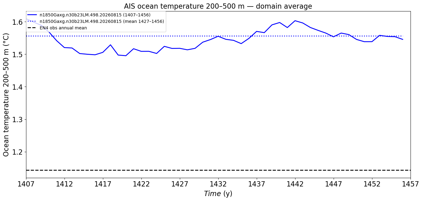
Time series: domain-averaged 200–500 m temperature vs. time with obs reference line.

# Colormaps
my_cmap = plt.get_cmap("RdBu_r")
my_cmap_diff = plt.get_cmap("bwr")

# Colorbar bounds for AW temperature (°C)
vmin = -1.0
vmax = 4.0
vmin_diff = -4.0
vmax_diff = 4.0

fig, axes = plt.subplots(1, 3, sharey=True, figsize=[22, 9])

utils.plot_contour_temp(
    ocean_temp_case_climo,
    fig,
    axes[0],
    f"Ocean temp 200–500 m (°C)\nMean {climo_first_year:04d}–{last_year:04d}",
    vmin, vmax, my_cmap,
)
axes[0].set_xlabel(case_name, fontsize=10)

utils.plot_contour_temp(
    obs_aw,
    fig,
    axes[1],
    f"{obs_dataset.upper()} observed AW temp 200–500 m (°C)\nAnnual mean climatology",
    vmin, vmax, my_cmap,
    show_cbar=False,
)

utils.plot_contour_temp(
    xr.DataArray(ocean_temp_case_climo.data - obs_aw.data, dims=["glc1Exp_ny", "glc1Exp_nx"]),
    fig,
    axes[2],
    f"Bias (CESM − {obs_dataset.upper()})\nOcean temp 200–500 m (°C)",
    vmin_diff, vmax_diff, my_cmap_diff,
)

# Comparing ocean temp 200–500 m: new run vs base case
if base_case_name:
    fig, axes = plt.subplots(1, 3, sharey=True, figsize=[22, 9])

    utils.plot_contour_temp(
        ocean_temp_case_climo,
        fig,
        axes[0],
        f"Ocean temp 200–500 m (°C)\nMean {climo_first_year:04d}–{last_year:04d}",
        vmin, vmax, my_cmap,
    )
    axes[0].set_xlabel(case_name, fontsize=10)

    utils.plot_contour_temp(
        ocean_temp_base_climo,
        fig,
        axes[1],
        f"Ocean temp 200–500 m (°C)\nMean {base_climo_first_year:04d}–{base_last_year:04d}",
        vmin, vmax, my_cmap,
        show_cbar=False,
    )
    axes[1].set_xlabel(base_case_name, fontsize=10)

    utils.plot_contour_temp(
        xr.DataArray(
            ocean_temp_case_climo.data - ocean_temp_base_climo.data,
            dims=["glc1Exp_ny", "glc1Exp_nx"],
        ),
        fig,
        axes[2],
        "Ocean temp 200–500 m difference (CESM − base) (°C)",
        vmin_diff, vmax_diff, my_cmap_diff,
    )

# Time series: domain-averaged AW temperature 200-500 m
time = np.arange(first_year, last_year + 1)
nt = len(time)

avg_temp_case_ts = np.full(nt, avg_temp_case_climo)

if base_case_name:
    base_time = (
        np.arange(base_first_year, base_last_year + 1) + first_year - base_first_year
    )
    full_time = np.arange(time[0], max(time[-1], base_time[-1]) + 1)
    base_nt = len(base_time)
    avg_temp_base_ts = np.full(base_nt, avg_temp_base_climo)
else:
    full_time = time

n_years = full_time[-1] - full_time[0] + 1
tick_step = 5 if n_years <= 100 else 10 if n_years <= 200 else 20
x_ticks = np.arange(full_time[0], full_time[-1] + tick_step, tick_step)
sizefont = 16

plt.figure(figsize=(16, 7))
plt.subplot(111)

utils.plot_line(
    avg_temp_case,
    time,
    line="-",
    color="blue",
    label=f"{case_name} ({first_year:04d}–{last_year:04d})",
    linewidth=2,
)
utils.plot_line(
    avg_temp_case_ts,
    time,
    line=":",
    color="blue",
    label=f"{case_name} (mean {climo_first_year:04d}–{last_year:04d})",
    linewidth=2,
)

if base_case_name:
    utils.plot_line(
        avg_temp_base,
        base_time,
        line="-",
        color="red",
        label=f"{base_case_name} ({base_first_year:04d}–{base_last_year:04d})",
        linewidth=2,
    )
    utils.plot_line(
        avg_temp_base_ts,
        base_time,
        line=":",
        color="red",
        label=f"{base_case_name} (mean {base_climo_first_year:04d}–{base_last_year:04d})",
        linewidth=2,
    )

plt.axhline(
    obs_mean,
    color="black",
    linestyle="--",
    linewidth=2,
    label=f"{obs_dataset.upper()} obs annual mean",
)

plt.xlim([first_year, last_year])
plt.xticks(x_ticks, x_ticks, fontsize=sizefont)
plt.xlabel(r"$Time$ (y)", fontsize=sizefont)
plt.ylabel("Ocean temperature 200–500 m (°C)", fontsize=sizefont)
plt.yticks(fontsize=sizefont)
plt.legend(loc="upper left", ncol=1, frameon=True, borderaxespad=0)
plt.title("AIS ocean temperature 200–500 m — domain average", fontsize=sizefont);