Antarctic Ice Sheet SMB comparison with MAR

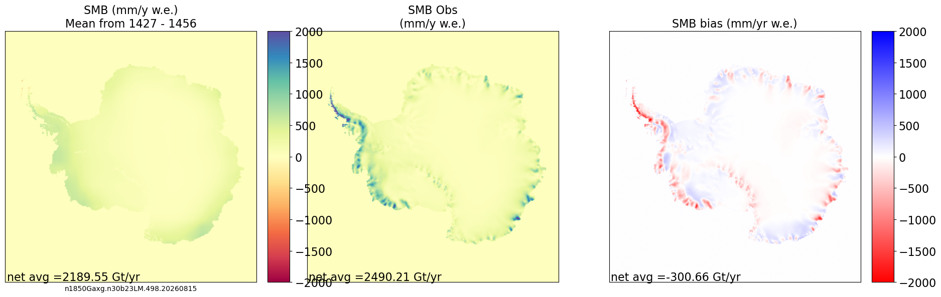
This notebook compares the downscaled output of surface mass balance (SMB) over the Antarctic ice sheet (AIS) to the regional model MAR. In what follows, we interchangeably call the MAR data “observation”.
Note1: the MAR data are processed as a climatology spanning 1960-1999.
Note2: the MAR data are available at a uniform resolution of 1km using the same projection as the CISM grid. This notebook requires the interpolation of the MAR data on the CISM grid. The interpolation is done in this notebook (for now) to allow for the eventuality of the CISM grid or the MAR grid to change in the future.
creation: 05-26-24
contact: Gunter Leguy (gunterl@ucar.edu)

Show code cell source

Hide code cell source

# Import packages
import os

import numpy as np
import matplotlib.pyplot as plt
from scipy.interpolate import RegularGridInterpolator
import xarray as xr

from cupid_utils.glc import utils

# to display figures in notebook after executing the code.
%matplotlib inline

Parameter configuration

Some parameters are set in CUPiD’s config.yml file, others are derived from these parameters.

Show code cell source

Hide code cell source

# Parameter Defaults

CESM_output_dir = ""
case_name = ""  # case name
climo_nyears = 0  # number of years to load for time series
end_date = ""

base_case_output_dir = None
base_case_name = None
base_end_date = None
base_climo_nyears = 0  # number of years to load for base case time series

obs_data_dir = ""  # global directory containing observed dataset
obs_path = ""  # specific directory containing observed dataset
obs_name = ""  # file name for observed dataset

# Climatology period for spatial map
map_climo_nyears = 30  # last N years used for climatology map and bias

# Parameters
case_name = "n1850Gaxg.n30b23LM.498.20260815"
base_case_name = ""
CESM_output_dir = "/datalake/NS9560K/noresm3/cases"
start_date = "1407-01-01"
end_date = "1456-01-01"
base_start_date = "0000-01-01"
base_end_date = "0000-01-01"
lc_kwargs = {"threads_per_worker": 1}
serial = False
obs_path = (
    "/nird/datapeak/NS9560K/users/heig/CUPiD_testdata/diagnostic_framework/SMB_data"
)
obs_name = "SMB_MARv3.14-AIS-yearly-ERA5-1979-2009ltm_08000m.nc"
climo_nyears = 50
base_climo_nyears = 0
subset_kwargs = {}
product = "/nird/datapeak/NS9560K/users/heig/CUPiD_Apr/examples/glc_metrics/computed_notebooks//glc/Antarctica_SMB_visual_compare_obs.ipynb"

Show code cell source

Hide code cell source

# Want some base case parameter defaults to equal control case values
if base_case_name is not None:
    if base_case_output_dir is None:
        base_case_output_dir = CESM_output_dir

    if base_end_date is None:
        base_end_date = end_date

    if base_climo_nyears == 0:
        base_climo_nyears = climo_nyears

Show code cell source

Hide code cell source

last_year = int(end_date.split("-")[0])

case_init_file = os.path.join(
    obs_data_dir, obs_path, "antarctica_8km_epsg3031_c20250403.nc"
)  # name of glc file output

case_path = os.path.join(
    CESM_output_dir, case_name, "cpl", "hist"
)  # path to glc output
case_file = os.path.join(
    case_path, f"{case_name}.cpl.hx.1yr2glc.{last_year:04d}-01-01-00000.nc"
)  # name of glc file output
obs_file = os.path.join(
    obs_data_dir, obs_path, obs_name
)  # name of observed dataset file

if base_case_name is not None:
    base_last_year = int(base_end_date.split("-")[0])
    base_case_path = os.path.join(
        base_case_output_dir, base_case_name, "cpl", "hist"
    )  # path to cpl output
    base_file = os.path.join(
        base_case_path,
        f"{base_case_name}.cpl.hx.1yr2glc.{base_last_year:04d}-01-01-00000.nc",
    )  # name of last cpl simulation output

Set up grid

Read in the grid data, compute resolution and other grid-specific parameters

Show code cell source

Hide code cell source

## Get grid from initial_hist stream
thk_init_da = xr.open_dataset(case_init_file).isel(time=0)["thk"]
mask = thk_init_da.data[:, :] == 0

# Shape of array is (ny, nx)
grid_dims = thk_init_da.shape

Show code cell source

Hide code cell source

# Constants
res = np.abs(
    thk_init_da["x1"].data[1] - thk_init_da["x1"].data[0]
)  # CISM output resolution

rhow = 1000  # water density kg/m3
kg_to_Gt = 1e-12  # Converting kg to Gt
mm_to_Gt = rhow * 1e-3 * res**2 * kg_to_Gt  # converting mm/yr to Gt/yr

Show code cell source

Hide code cell source

params = {
    "grid_dims": grid_dims,
    "mm_to_Gt": mm_to_Gt,
    "mask": mask,
}

Make datasets

Read in observations and CESM output. Also do necessary computations (global mean for time series, temporal mean for climatology).

Show code cell content

Hide code cell content

# Load all available years for time series; climatology uses last map_climo_nyears years
smb_case = utils.read_cesm_smb(case_path, case_name, 'AIS', last_year, climo_nyears, params)
if smb_case is None:
    raise RuntimeError(f"AIS not present in {case_name!r} output — skipping notebook.")
smb_case_climo = smb_case.isel(time=slice(-map_climo_nyears, None)).mean("time")

if base_case_name:
    smb_base_case = utils.read_cesm_smb(
        base_case_path, base_case_name, 'AIS', base_last_year, base_climo_nyears, params
    )
    smb_base_climo = smb_base_case.isel(time=slice(-map_climo_nyears, None)).mean("time")

number of years used in climatology =  50

Show code cell source

Hide code cell source

# Interpolating the observed data onto the CISM grid
smb_obs_da = xr.open_dataset(obs_file).isel(time=0)["SMB"]

# Defining the interpolation functions
myInterpFunction_smb_obs = RegularGridInterpolator(
    (smb_obs_da["x"].data, smb_obs_da["y"].data),
    smb_obs_da.data.transpose(),
    method="linear",
    bounds_error=False,
    fill_value=None,
)

# Initializing the glacier ID variable
smb_obs_climo = xr.DataArray(np.zeros(grid_dims), dims=["glc1Exp_ny", "glc1Exp_nx"])

# Performing the interpolation
for j in range(grid_dims[0]):
    point_y = np.zeros(grid_dims[1])
    point_y[:] = thk_init_da["y1"].data[j]
    pts = (thk_init_da["x1"].data[:], point_y[:])
    smb_obs_climo.data[j, :] = myInterpFunction_smb_obs(pts)

# Filtering out fill values
smb_obs_climo.data = np.where(
    np.logical_or(mask, smb_obs_climo > 1e20), 0, smb_obs_climo
)

Show code cell source

Hide code cell source

# Integrated SMB time series
first_year = last_year - len(smb_case["time"]) + 1
climo_first_year = last_year - map_climo_nyears + 1
avg_smb_case_climo = smb_case.sum(["glc1Exp_ny", "glc1Exp_nx"]) * params["mm_to_Gt"]

if base_case_name:
    base_first_year = base_last_year - len(smb_base_case["time"]) + 1
    base_climo_first_year = base_last_year - map_climo_nyears + 1
    avg_smb_base_case_climo = (
        smb_base_case.sum(["glc1Exp_ny", "glc1Exp_nx"]) * params["mm_to_Gt"]
    )

Generate plots

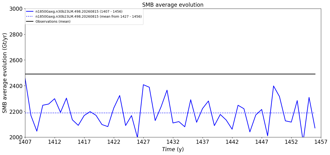
Map comparing CESM to observation, possibly map comparing CESM to older case, and time series of spatial mean SMB.

Show code cell source

Hide code cell source

# Comparing SMB new run vs obs

my_cmap = plt.get_cmap("Spectral")
my_cmap_diff = plt.get_cmap("bwr_r")

vmin = -2000
vmax = 2000

fig, ax = plt.subplots(1, 3, sharey=True, figsize=[22, 9])

utils.plot_contour(
    smb_case_climo,
    fig,
    ax[0],
    None,
    f"SMB (mm/y w.e.)\nMean from {climo_first_year:04d} - {last_year:04d}",
    vmin,
    vmax,
    my_cmap,
    mm_to_Gt,
)
ax[0].set_xlabel(case_name, fontsize=10)

utils.plot_contour(
    smb_obs_climo,
    fig,
    ax[1],
    None,
    "SMB Obs\n(mm/y w.e.)",
    vmin,
    vmax,
    my_cmap,
    mm_to_Gt,
    show_cbar=False,
)

utils.plot_contour(
    smb_case_climo - smb_obs_climo,
    fig,
    ax[2],
    None,
    "SMB bias (mm/yr w.e.)",
    vmin,
    vmax,
    my_cmap_diff,
    mm_to_Gt,
)

Show code cell source

Hide code cell source

# Comparing SMB new run vs base case
if base_case_name:
    my_cmap = plt.get_cmap("Spectral")
    my_cmap_diff = plt.get_cmap("bwr_r")

    vmin = -2000
    vmax = 2000

    fig, ax = plt.subplots(1, 3, sharey=True, figsize=[22, 9])

    utils.plot_contour(
        smb_case_climo,
        fig,
        ax[0],
        None,
        f"SMB (mm/y w.e.)\nMean from {climo_first_year:04d} - {last_year:04d}",
        vmin,
        vmax,
        my_cmap,
        mm_to_Gt,
    )
    ax[0].set_xlabel(case_name, fontsize=10)

    utils.plot_contour(
        smb_base_climo,
        fig,
        ax[1],
        None,
        f"SMB (mm/y w.e.)\nMean from {base_climo_first_year:04d} - {base_last_year:04d}",
        vmin,
        vmax,
        my_cmap,
        mm_to_Gt,
        show_cbar=False,
    )
    ax[1].set_xlabel(base_case_name, fontsize=10)

    utils.plot_contour(
        smb_case_climo - smb_base_climo,
        fig,
        ax[2],
        None,
        "SMB difference (mm/yr w.e.)",
        vmin,
        vmax,
        my_cmap_diff,
        mm_to_Gt,
    )

Show code cell source

Hide code cell source

# Plotting the SMB spatially averaged time series

time = np.arange(first_year, last_year + 1)
full_time = time
if base_case_name:
    base_time = (
        np.arange(base_first_year, base_last_year + 1) + first_year - base_first_year
    )
    base_nt = len(base_time)
    full_time = np.arange(time[0], max(time[-1], base_time[-1]) + 1)
nt = len(time)

avg_smb_obs_timeseries = np.zeros(len(full_time))
avg_smb_case_timeseries = np.zeros(nt)
if base_case_name:
    avg_smb_base_timeseries = np.zeros(base_nt)

avg_smb_obs_timeseries[:] = np.round(smb_obs_climo.sum() * mm_to_Gt, 2)
avg_smb_case_timeseries[:] = np.round(smb_case_climo.sum() * mm_to_Gt, 2)
if base_case_name:
    avg_smb_base_timeseries[:] = np.round(smb_base_climo.sum() * mm_to_Gt, 2)

n_years = full_time[-1] - full_time[0] + 1
tick_step = 5 if n_years <= 100 else 10 if n_years <= 200 else 20
x_ticks = np.arange(full_time[0], full_time[-1] + tick_step, tick_step)
tickx = x_ticks

ymin = 2000
ymax = 3000
y_step = 100
y_ticks = np.arange(ymin, ymax + y_step, y_step)

plt.figure(figsize=(16, 7))
plt.subplot(111)
utils.plot_line(
    avg_smb_case_climo,
    time,
    line="-",
    color="blue",
    label=f"{case_name} ({first_year:04d} - {last_year:04d})",
    linewidth=2,
)
utils.plot_line(
    avg_smb_case_timeseries[:],
    time,
    line=":",
    color="blue",
    label=f"{case_name} (mean from {climo_first_year:04d} - {last_year:04d})",
    linewidth=2,
)
if base_case_name:
    utils.plot_line(
        avg_smb_base_case_climo,
        base_time,
        line="-",
        color="red",
        label=f"{base_case_name} ({base_first_year:04d} - {base_last_year:04d})",
        linewidth=2,
    )
    utils.plot_line(
        avg_smb_base_timeseries[:],
        base_time,
        line=":",
        color="red",
        label=f"{base_case_name} (mean from {base_climo_first_year:04d} - {base_last_year:04d})",
        linewidth=2,
    )
utils.plot_line(
    avg_smb_obs_timeseries[:],
    full_time,
    line="-",
    color="black",
    label="Observations (mean)",
    linewidth=2,
)

sizefont = 16
plt.xlim([first_year, last_year])
plt.xticks(x_ticks, tickx, fontsize=sizefont)
plt.xlabel(r"$Time$ (y)", fontsize=sizefont)
plt.ylabel("SMB average evolution (Gt/yr)", multialignment="center", fontsize=sizefont)
plt.ylim([ymin, ymax])
plt.yticks(fontsize=sizefont)
plt.legend(loc="upper left", ncol=1, frameon=True, borderaxespad=0)
plt.title("SMB average evolution", fontsize=sizefont);