Greenland Ice Sheet thickness change vs BedMachine

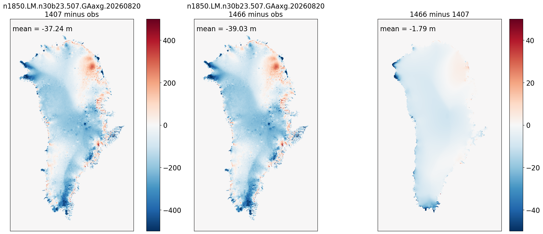
This notebook compares two snapshots of Greenland ice thickness (GrIS) from a CESM/CISM run to present-day observed ice thickness (BedMachine), and to each other.
Three panels are shown: model-minus-obs at the start of the analysis period, model-minus-obs at the end of the analysis period, and end-minus-start (pure model thickness change over the period). No time averaging is performed — each panel uses single-year snapshots.

Show code cell source

Hide code cell source

# Import packages
import os

import xarray as xr
import matplotlib.pyplot as plt

from cupid_utils.glc import utils

# to display figures in notebook after executing the code.
%matplotlib inline

Parameter configuration

Some parameters are set in CUPiD’s config.yml file, others are derived from these parameters.

Show code cell source

Hide code cell source

# Parameter Defaults

CESM_output_dir = ""
case_name = ""  # case name
start_date = ""
end_date = ""

obs_data_dir = ""  # global directory containing observed dataset
obs_path = ""  # specific directory containing observed dataset
obs_name = ""  # file name for observed dataset

# Parameters
case_name = "n1850.LM.n30b23.507.GAaxg.20260820"
base_case_name = ""
CESM_output_dir = "/datalake/NS9560K/noresm3/cases"
start_date = "1407-01-01"
end_date = "1466-01-01"
base_start_date = "0000-01-01"
base_end_date = "0000-01-01"
lc_kwargs = {"threads_per_worker": 1}
serial = False
obs_path = (
    "/nird/datapeak/NS5011K/users/mali/CISM/GrIS/Database7/Obs/Geometry/BM6/Ready"
)
obs_name = "BM6_sm06_v1_i04000m.nc"
subset_kwargs = {}
product = "/nird/datapeak/NS9560K/users/heig/CUPiD_Apr/examples/glc_thk_test/computed_notebooks//glc/Greenland_thickness_diff.ipynb"

Show code cell source

Hide code cell source

start_year = int(start_date.split("-")[0])
end_year = int(end_date.split("-")[0])

case_path = os.path.join(
    CESM_output_dir, case_name, "glc", "hist"
)  # path to CISM component history output

obs_file = os.path.join(
    obs_data_dir, obs_path, obs_name
)  # name of observed dataset file

Make datasets

Read in the start-year and end-year model snapshots and the observed thickness, and compute the three difference fields.

Show code cell content

Hide code cell content

# Read single-year model thickness snapshots (no time averaging)
thk_start = utils.read_cesm_thk(case_path, case_name, 'GrIS', start_year)
thk_end = utils.read_cesm_thk(case_path, case_name, 'GrIS', end_year)
if thk_start is None or thk_end is None:
    raise RuntimeError(f"GrIS not present in {case_name!r} output — skipping notebook.")

# Observed present-day thickness (already regridded to the CISM GrIS grid)
thk_obs = xr.open_dataset(obs_file).isel(time=0)["thk"]

Show code cell source

Hide code cell source

# Compute the three difference fields. Obs is pre-regridded to the same
# CISM grid as the model output, but x1/y1 coordinate values are not
# guaranteed to be bit-identical between files, so difference on .data
# directly rather than relying on xarray coordinate alignment.
diff_start_obs = xr.DataArray(thk_start.data - thk_obs.data, dims=thk_start.dims)
diff_end_obs = xr.DataArray(thk_end.data - thk_obs.data, dims=thk_start.dims)
diff_end_start = xr.DataArray(thk_end.data - thk_start.data, dims=thk_start.dims)

Generate plots

Three-panel map: model-minus-obs at the start of the period, model-minus-obs at the end of the period, and end-minus-start.

Show code cell source

Hide code cell source

# Comparing model thickness to observations at start/end of period, and to itself.
# The obs-comparison panels (1-2) and the model-drift panel (3) get separate
# color scales: model-vs-obs bias is typically O(10-100 m), while model drift
# over a single run can be much smaller and would be invisible on the obs scale.
# Panels 1-2 share one colorbar (same scale, like the SMB case-vs-obs maps);
# panel 3 gets its own.

my_cmap_diff = plt.get_cmap("RdBu_r")

vmin_obs = -500
vmax_obs = 500

vmin_drift = -50
vmax_drift = 50

fig, ax = plt.subplots(1, 3, sharey=True, figsize=[22, 9])

utils.plot_contour_temp(
    diff_start_obs,
    fig,
    ax[0],
    f"{case_name}\n{start_year} minus obs",
    vmin_obs,
    vmax_obs,
    my_cmap_diff,
    units="m",
    left=0.35,
)

utils.plot_contour_temp(
    diff_end_obs,
    fig,
    ax[1],
    f"{case_name}\n{end_year} minus obs",
    vmin_obs,
    vmax_obs,
    my_cmap_diff,
    units="m",
    show_cbar=False,
)

utils.plot_contour_temp(
    diff_end_start,
    fig,
    ax[2],
    f"{end_year} minus {start_year}",
    vmin_drift,
    vmax_drift,
    my_cmap_diff,
    units="m",
    left=0.89,
)